Low-pass Filter Implementation

N = 1024;              % signal length
x = [1 zeros(1, N-1)]; % impulse
y = [1 zeros(1, N-1)]; % output buffer

for n=2:N
  y(n) = x(n)+x(n-1);  % impulse response
end

Y = fft(y);          % frequency response
Y = abs(Y(1:N/2));   % amplitude response (positive frequencies)
fn = [0:N/2-1]/N;    % frequency axis

subplot(211); plot(fn, Y); grid;
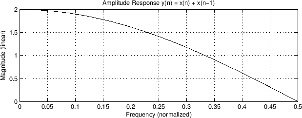
title('Amplitude Response y(n) = x(n) + x(n-1)');
xlabel('Frequency (normalized)');
ylabel('Magnitude (linear)');

Figure 6: Magnitude response for the filter y(n) = x(n) + x(n-1).